Example 1: The BS Disease

Uh oh! You just learned that you tested positive for the very serious BS disease. It affects 0.1% of the population. The test for the disease is 99% accurate. What are the chances that you actually have BS?

Bayes’ Theorem

\[ P(BS \mid test) = \frac{P(test \mid BS) \, P(BS)}{P(test)} \]

The test is 99% accurate, so \(P(test \mid BS) = 0.99\). BS prevalence is 0.1%, so \(P(BS) = 0.001\). We want to know chance of testing positive, \(P(test)\), so we reformulate like so:

\[P(test) = P(BS) \times P(test \mid BS) + P(-BS) \times P(test \mid -BS)\]

So we plug and chug:

\[P(BS \mid test) = \frac{0.99 \times 0.001}{0.001 \times 0.99 + (1 - 0.001) \times (1 - 0.99)}\]

You tested positive, but there’s only a 9% chance that you actually have BS.

What’s the point?

Bayes’ Theorem rocks!

\[ \begin{aligned} \overbrace{p(\theta | \text{Data})}^{\text{posterior}} &= \frac{\overbrace{p(\text{Data} | \theta)}^{\text{likelihood}} \times \overbrace{p(\theta)}^{\text{prior}}}{\underbrace{p(\text{Data})}_{\text{marginal likelihood}}} \\ &\propto p(\text{Data} | \theta) \times p(\theta) \\ \end{aligned} \]

We can confront our model with the data and incorporate our prior understanding to draw inference about parameters of interest.

Example 2: A/B Testing

Stan

Probabilistic programming language
Implements fancy HMC algorithms
Written in C++ for speed
Interfaces for R (rstan), python (pystan), etc.
Active developers on cutting-edge of HMC research
Large user community

A/B Testing

Suppose your manager approaches you and says,

We’re testing an exciting new web feature! Version A has a red button, and version B has a green button. Which version yields more conversions?”

How can you answer this question?

The Data

df <- expand.grid(
  version = c("A", "B"), 
  converted = c("Yes", "No")
)
df$n_visitors <- c(1300, 1275, 120, 125)
df

  version converted n_visitors
1       A       Yes       1300
2       B       Yes       1275
3       A        No        120
4       B        No        125

The Model

The model of the experiment is an A/B test in which

\[ \begin{aligned} n_A &\sim \mathsf{Binomial}(N_A, \pi_A) & n_B &\sim \mathsf{Binomial}(N_B, \pi_B) \\ \pi_A &= \mathsf{InvLogit}(\eta_A) & \pi_B &= \mathsf{InvLogit}(\eta_B) \\ \eta_A &= \mathsf{Normal}(0, 2.5) & \eta_B &= \mathsf{Normal}(0, 2.5) \end{aligned} \]

Implementation in Stan

data {
  int<lower=1> visitors_A;
  int<lower=0> conversions_A;
  int<lower=1> visitors_B;
  int<lower=0> conversions_B;
}
parameters {
  real eta_A;
  real eta_B;
}
transformed parameters {
  real<lower=0., upper=1.> pi_A = inv_logit(eta_A);
  real<lower=0., upper=1.> pi_B = inv_logit(eta_B);
}
model {
  eta_A ~ normal(0., 2.5);
  eta_B ~ normal(0., 2.5);
  conversions_A ~ binomial(visitors_A, pi_A);
  conversions_B ~ binomial(visitors_B, pi_B);
}
generated quantities {
  real<lower=-1., upper=1.> pi_diff;
  real eta_diff;
  real lift;

  pi_diff = pi_B - pi_A;
  eta_diff = eta_B - eta_A;
  lift = (pi_B - pi_A) / pi_B;
}

Run and fit the model

abtest_data <- list(
  visitors_A = 1300,
  visitors_B = 1275,
  conversions_A = 120,
  conversions_B = 125
)

abtest_fit <- rstan::sampling(
  model, 
  data = abtest_data,
  chains = 1, 
  iter = 1000, 
  refresh = 0
)

Calculate the probability that \(\pi_A\)

pi_A <- drop(rstan::extract(abtest_fit, "pi_A")[[1]])
pi_B <- drop(rstan::extract(abtest_fit, "pi_B")[[1]])
mean(pi_A > pi_B)

[1] 0.314

mean(pi_A < pi_B)

[1] 0.686

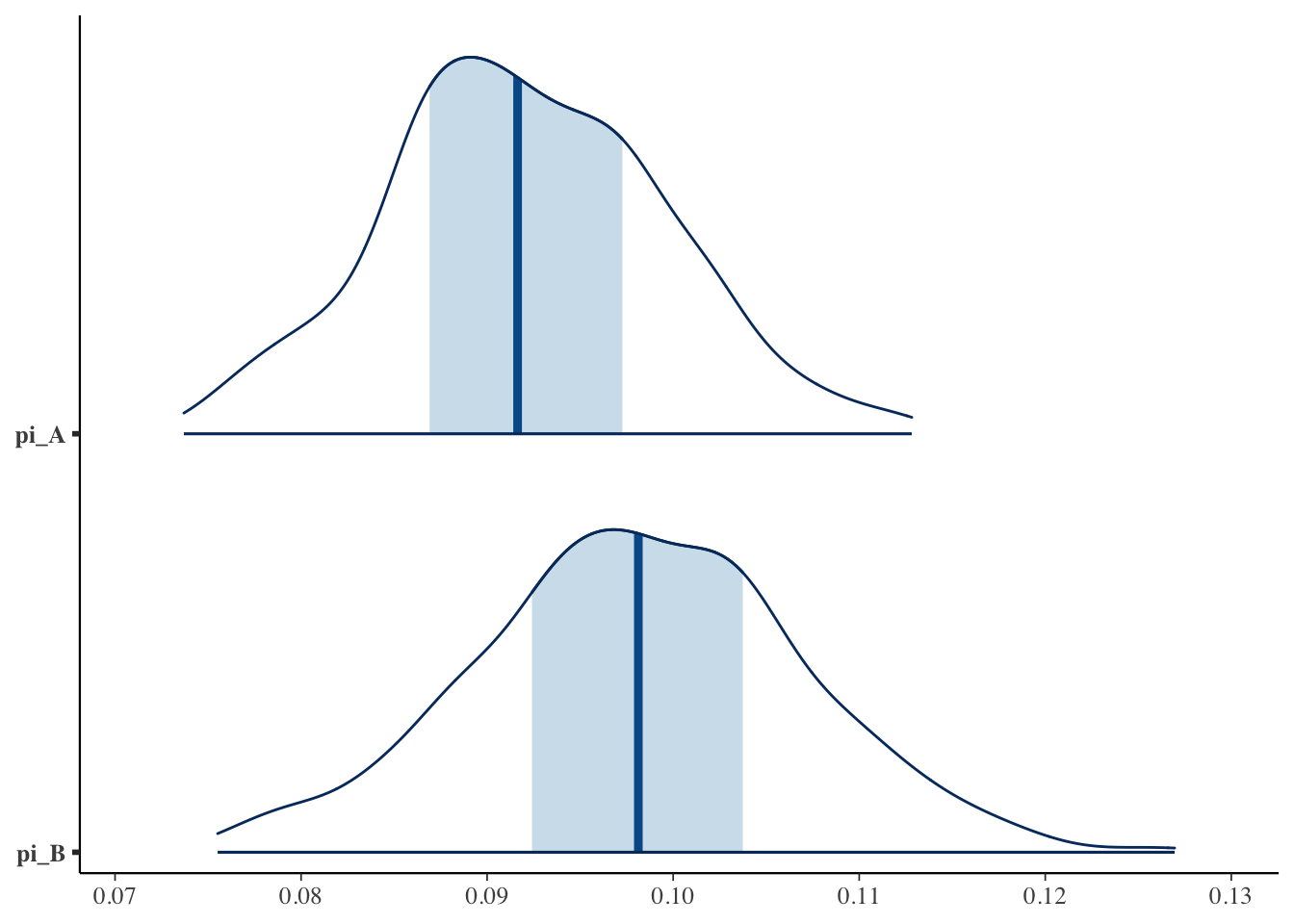
Looks like Version B wins!

Plot posteriors

posterior <- as.matrix(abtest_fit)
bayesplot::mcmc_areas(posterior, pars = c("pi_A", "pi_B"))