You’re running A/B tests on your app’s checkout flow. The current design (Control) is being tested against a redesigned version (Treatment). You collect data, run a t-test, and get your p-value. Simple enough.
But what if you want to test multiple variations simultaneously? What if you want to understand not just “did it change?” but “what kind of change matters?” This is where orthogonal contrasts come in—a powerful experimental design that lets you ask more sophisticated questions while maintaining statistical rigor.
The Traditional A/B Test: A Quick Review
Let’s set up a realistic scenario. You’re a product manager at a mobile commerce company, and you want to optimize your checkout button. Your current button says “Buy Now” with a blue background. You suspect that both the text and color might affect conversion rates.
In a traditional A/B test, you’d compare your current design against one alternative:
library(tidyverse)set.seed(42)# Simulate conversion data: 1000 users per groupn_per_group <-1000# Control: "Buy Now" blue button (baseline 12% conversion)# Treatment: "Complete Purchase" green button (14% conversion)control <-rbinom(n_per_group, 1, 0.12)treatment <-rbinom(n_per_group, 1, 0.14)# Traditional t-testt.test(treatment, control)
    Welch Two Sample t-test

data:  treatment and control
t = 0.92162, df = 1994, p-value = 0.3568
alternative hypothesis: true difference in means is not equal to 0
95 percent confidence interval:
 -0.01579114  0.04379114
sample estimates:
mean of x mean of y
    0.140     0.126
This tells us whether the treatment is different from control. But here’s the limitation: we changed two things at once (text and color). If the result is significant, we don’t know if it’s the text, the color, or their combination that drove the change.
The naive solution? Run separate tests: - Test 1: Blue “Buy Now” vs Blue “Complete Purchase” - Test 2: Blue “Buy Now” vs Green “Buy Now” - Test 3: Blue “Buy Now” vs Green “Complete Purchase”
But now you have a multiple comparisons problem, you need more users, and the tests aren’t efficiently designed.
Enter Orthogonal Contrasts
Orthogonal contrasts are a way to partition the variance in your experiment into independent, non-overlapping components. Instead of asking “is there any difference somewhere?”, you ask specific, pre-planned questions that together account for all the systematic variation in your data.
For our checkout button example, we can design a 2×2 factorial experiment:
Condition
Text
Color
A
Buy Now
Blue
B
Buy Now
Green
C
Complete Purchase
Blue
D
Complete Purchase
Green
With orthogonal contrasts, we can simultaneously test:
Main effect of Text: Does “Complete Purchase” perform differently than “Buy Now”?
Main effect of Color: Does green perform differently than blue?
Interaction: Does the effect of text depend on color (or vice versa)?
These three contrasts are orthogonal—mathematically independent—which means: - No multiple comparison penalty needed - Each contrast uses all the data efficiently - The sum of their effects equals the total treatment variance
The Math Behind Orthogonal Contrasts
For our four conditions (A, B, C, D), we can define contrast coefficients that sum to zero and are orthogonal to each other:
Contrast
A
B
C
D
Interpretation
Text
-1
-1
+1
+1
Complete Purchase vs Buy Now
Color
-1
+1
-1
+1
Green vs Blue
Interaction
+1
-1
-1
+1
Does text effect differ by color?
Two contrasts are orthogonal when the sum of the products of their coefficients equals zero: - Text × Color: (-1×-1) + (-1×1) + (1×-1) + (1×1) = 1 - 1 - 1 + 1 = 0 ✓ - Text × Interaction: (-1×1) + (-1×-1) + (1×-1) + (1×1) = -1 + 1 - 1 + 1 = 0 ✓ - Color × Interaction: (-1×1) + (1×-1) + (-1×-1) + (1×1) = -1 - 1 + 1 + 1 = 0 ✓
Implementing Orthogonal Contrasts in R
Let’s simulate the full factorial experiment:
set.seed(123)n_per_condition <-500# Define true effects (in probability scale)base_rate <-0.12text_effect <-0.02# "Complete Purchase" adds 2 percentage pointscolor_effect <-0.015# Green adds 1.5 percentage pointsinteraction_effect <-0.01# Extra boost when both changes are present# Generate data for each conditiondata <-tibble(condition =rep(c("A", "B", "C", "D"), each = n_per_condition),text =rep(c("Buy Now", "Buy Now", "Complete Purchase", "Complete Purchase"),each = n_per_condition ),color =rep(c("Blue", "Green", "Blue", "Green"), each = n_per_condition)) |>mutate(# Calculate true conversion probability for each conditiontrue_prob =case_when( condition =="A"~ base_rate, condition =="B"~ base_rate + color_effect, condition =="C"~ base_rate + text_effect, condition =="D"~ base_rate + text_effect + color_effect + interaction_effect ),converted =rbinom(n(), 1, true_prob) )# View the observed conversion ratesdata |>group_by(condition, text, color) |>summarise(n =n(),conversions =sum(converted),rate =mean(converted),.groups ="drop" ) |> knitr::kable(digits =3, caption ="Observed Conversion Rates by Condition")
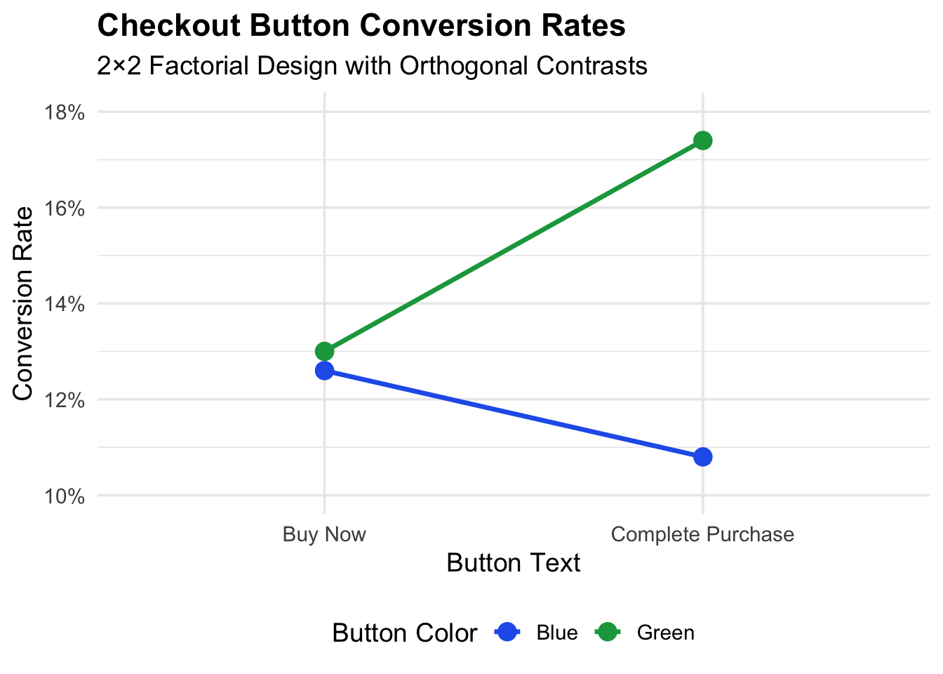
Observed Conversion Rates by Condition
condition
text
color
n
conversions
rate
A
Buy Now
Blue
500
63
0.126
B
Buy Now
Green
500
65
0.130
C
Complete Purchase
Blue
500
54
0.108
D
Complete Purchase
Green
500
87
0.174
Now let’s set up and test our orthogonal contrasts:
# Set up factors with proper codingdata <- data |>mutate(text_code =ifelse(text =="Complete Purchase", 1, -1),color_code =ifelse(color =="Green", 1, -1),interaction_code = text_code * color_code )# Fit the modelmodel <-lm(converted ~ text_code + color_code + interaction_code, data = data)summary(model)
Call:
lm(formula = converted ~ text_code + color_code + interaction_code,
    data = data)

Residuals:
   Min     1Q Median     3Q    Max
-0.174 -0.130 -0.126 -0.108  0.892

Coefficients:
                 Estimate Std. Error t value Pr(>|t|)
(Intercept)      0.134500   0.007618  17.657   <2e-16 ***
text_code        0.006500   0.007618   0.853   0.3936
color_code       0.017500   0.007618   2.297   0.0217 *
interaction_code 0.015500   0.007618   2.035   0.0420 *
---
Signif. codes:  0 '***' 0.001 '**' 0.01 '*' 0.05 '.' 0.1 ' ' 1

Residual standard error: 0.3407 on 1996 degrees of freedom
Multiple R-squared:  0.005058,  Adjusted R-squared:  0.003562
F-statistic: 3.382 on 3 and 1996 DF,  p-value: 0.01755
Let’s interpret these results more clearly:
# Extract coefficients and compute confidence intervalscoef_summary <- broom::tidy(model, conf.int =TRUE) |>filter(term !="(Intercept)") |>mutate(term =case_when( term =="text_code"~"Text Effect", term =="color_code"~"Color Effect", term =="interaction_code"~"Interaction" ),# Convert to percentage points (estimates are on 0-1 scale,# and coded -1/+1 so multiply by 2 for full effect)effect_pct = estimate *2*100,ci_low_pct = conf.low *2*100,ci_high_pct = conf.high *2*100 ) |>select(Contrast = term,`Effect (pct pts)`= effect_pct,`95% CI Low`= ci_low_pct,`95% CI High`= ci_high_pct,`p-value`= p.value )knitr::kable(coef_summary, digits =3, caption ="Orthogonal Contrast Results")
The non-parallel lines indicate an interaction effect: the benefit of green over blue is larger when combined with “Complete Purchase” text.
Why Orthogonal Contrasts Are More Powerful
Let’s demonstrate the power advantage with a simulation:
# Power simulation: compare traditional sequential tests vs orthogonal contrastssimulate_experiment <-function(n_per_condition, true_text_effect =0.02) { base_rate <-0.12 color_effect <-0.015 interaction_effect <-0.005 data <-tibble(condition =rep(c("A", "B", "C", "D"), each = n_per_condition),text =rep(c("Buy Now", "Buy Now", "Complete Purchase", "Complete Purchase"),each = n_per_condition ),color =rep(c("Blue", "Green", "Blue", "Green"), each = n_per_condition) ) |>mutate(true_prob =case_when( condition =="A"~ base_rate, condition =="B"~ base_rate + color_effect, condition =="C"~ base_rate + true_text_effect, condition =="D"~ base_rate + true_text_effect + color_effect + interaction_effect ),converted =rbinom(n(), 1, true_prob),text_code =ifelse(text =="Complete Purchase", 1, -1),color_code =ifelse(color =="Green", 1, -1) )# Orthogonal contrast approach model <-lm( converted ~ text_code + color_code + text_code:color_code,data = data ) orthogonal_p <-summary(model)$coefficients["text_code", "Pr(>|t|)"]# Traditional approach: just compare A vs C (same color, different text) traditional_p <-t.test( data$converted[data$condition =="C"], data$converted[data$condition =="A"] )$p.valuec(orthogonal = orthogonal_p <0.05, traditional = traditional_p <0.05)}# Run simulationset.seed(456)n_sims <-1000results <-replicate(n_sims, simulate_experiment(n_per_condition =300))power_comparison <-tibble(Method =c("Orthogonal Contrasts", "Traditional A/B Test"),Power =c(mean(results["orthogonal", ]), mean(results["traditional", ])),`Sample Size`=c("300 × 4 = 1200 total", "300 × 2 = 600 total"))knitr::kable( power_comparison,digits =3,caption ="Statistical Power Comparison (detecting 2 pct pt text effect)")
Statistical Power Comparison (detecting 2 pct pt text effect)
Method
Power
Sample Size
Orthogonal Contrasts
0.195
300 × 4 = 1200 total
Traditional A/B Test
0.100
300 × 2 = 600 total
The orthogonal contrast approach has higher power for detecting the text effect because it uses all the data efficiently. The traditional approach only uses conditions A and C, throwing away half the information.
Even more importantly, the orthogonal design answers three questions (text, color, interaction) for roughly the cost of one traditional test with equivalent power.
When to Use Orthogonal Contrasts
Orthogonal contrasts are ideal when:
You have multiple factors to test: Instead of running sequential A/B tests, design a factorial experiment upfront.
You care about interactions: Traditional A/B tests can’t detect interactions. If the effect of one change depends on another, you’ll miss it entirely.
You want to maximize information per user: In products with limited traffic, orthogonal designs extract more insights from fewer observations.
You have specific hypotheses: Orthogonal contrasts require pre-planned questions. If you’re just exploring, they may not be appropriate.
Practical Tips for Implementation
1. Plan your contrasts before collecting data. Post-hoc contrasts aren’t truly orthogonal and require multiple comparison corrections.
2. Balance your sample sizes. Orthogonal contrasts work best with equal n per condition. Unbalanced designs lose the clean independence property.
3. Limit the number of factors. A 2×2 design has 4 conditions. A 2×2×2 has 8. A 3×3×3 has 27. Designs get unwieldy quickly.
4. Consider effect coding vs. dummy coding. Effect coding (-1, +1) gives you main effects averaged across other conditions. Dummy coding (0, 1) gives you simple effects.
# Quick reference: setting up contrasts in R# For a 2x2 design, you can use contr.sum for automatic effect codingdata_factored <- data |>mutate(text_factor =factor(text),color_factor =factor(color) )# Set contrasts to sum-to-zero (effect coding)contrasts(data_factored$text_factor) <-contr.sum(2)contrasts(data_factored$color_factor) <-contr.sum(2)# This model is equivalent to our manual codingmodel_auto <-lm(converted ~ text_factor * color_factor, data = data_factored)summary(model_auto)
Call:
lm(formula = converted ~ text_factor * color_factor, data = data_factored)

Residuals:
   Min     1Q Median     3Q    Max
-0.174 -0.130 -0.126 -0.108  0.892

Coefficients:
                            Estimate Std. Error t value Pr(>|t|)
(Intercept)                 0.134500   0.007618  17.657   <2e-16 ***
text_factor1               -0.006500   0.007618  -0.853   0.3936
color_factor1              -0.017500   0.007618  -2.297   0.0217 *
text_factor1:color_factor1  0.015500   0.007618   2.035   0.0420 *
---
Signif. codes:  0 '***' 0.001 '**' 0.01 '*' 0.05 '.' 0.1 ' ' 1

Residual standard error: 0.3407 on 1996 degrees of freedom
Multiple R-squared:  0.005058,  Adjusted R-squared:  0.003562
F-statistic: 3.382 on 3 and 1996 DF,  p-value: 0.01755
Conclusion
Traditional A/B testing is fine for simple, single-factor experiments. But as your experimentation program matures, you’ll want to test multiple factors simultaneously and understand how they interact. Orthogonal contrasts provide a rigorous, efficient framework for doing exactly that.
The key insights: - Orthogonal contrasts partition variance into independent components - No multiple comparison penalties needed for pre-planned orthogonal contrasts - Higher statistical power by using all data for each contrast - Interactions are testable, revealing synergies (or conflicts) between changes
Next time you’re designing an experiment with multiple variations, consider whether orthogonal contrasts might give you more insight than a simple A/B test. Your statistical power—and your users—will thank you.